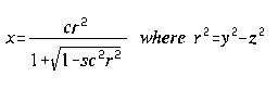
 The curvature c is specified
by 1/(radius of curvature at the center). The shape factor s can be:
The curvature c is specified
by 1/(radius of curvature at the center). The shape factor s can be:
CALC_LENS,filename [,optional keyword parameters]The program can also be run in a batch file (i.e. non-interactively). This is done by listing lines of the same form as the interactive command shown above. The batch file could look like this:
CALC_LENS,'infile1'
CALC_LENS,'infile2'
CALC_LENS,'infile2',num_rays=1001,outfile='infile2.1001.out'
This would run three different parameter sets. The files 'infile1' and 'infile2' would contain the parameters. The third run would be modified from the second by tracing 1001 rays instead of whatever value was in 'infile2' and then saving the results in 'infile2.1001.out' instead of 'infile2.out'.
If the above three lines were saved in the file 'batch', then the command to run the batch file would be:
wave < batch >& batch.err &This tells the computer to run PV-WAVE using the file 'batch' as input. The trailing ampersand puts the process in the background, so you can continue using the computer for other tasks. Note, however, that if only one license for PV-WAVE is available, then PV-WAVE can't be run while this batch file is running. The ">& batch.err" stores the output of the program that would normally go to the screen to the file "batch.err". Timing information and errors will be stored in that file. The actual results of the program will be stored in the file named by /outfile, if specified, or by the input file name with '.out' appended to the end if /outfile isn't specified.
The filename parameter is the file name of a parameter file which contains information on the lens system and the type of calculation desired. The optional keyword parameters supersede the values stored in the parameter file(s). The available keyword parameters are:
If /outfile is set, then the output file name will be the input file name with ".out" appended. It can also be set to a string, in which case that will be used as the output file name. The output file stores the results of pressure calculations, so is only applicable when pressure calculations are performed.
If /savefile is set, then the save file name will be the input file name with ".save" appended. It can also be set to a string, in which case that will be used as the save file name. The save file stores the results of the ray tracing calculations, not the results of pressure calculations.
If /logfile is set, then the log file name will be "batch.log". It can also be set to a string, in which case that will be used as the log file name. The log file stores information on the progress of the calculation and the values being used. It is useful for debugging lens parameter files and viewing the progress of batch jobs, as well as storing the results of maxima search.
/num_rays sets or supersedes the number of rays which will be traced in the ray-tracing calculations. Similarly, /num_rings sets or supersedes the number of hexapolar rings in 3-D ray tracing. In 3-D ray tracing, the rays are arranged in hexapolar rings. There is 1 ray in the center, 6 rays in the first ring, 12 in the second, 18 in the third, etc. The rays in each ring are evenly distributed around the center of the lens. This results in 1+3*num_rings*(num_rings+1) total rays traced.
/skip is used when a large number of rays are to be traced, but only some fraction are to be plotted. For example, num_rays=300, skip=10 will plot every tenth ray, for a total of 30 rays plotted.
/waterspeed sets the speed of sound in water (or other ambient medium). The sound speed in water can be either a speed in meters/second, or as the number 0.0. If /waterspeed is not specified or is set to 0, the water speed will be calculated using equation (1.2.1) from Clay & Medwin, Acoustical Oceanography, 1977:
WaterSpeed=1449.2+4.6T-0.055T^2+0.00029T^3+(1.34-0.010T)(Sal-35)+0.016Depthwhere T is the water temperature in degrees Celsius, Sal is the water salinity in parts per million, and Depth is the system depth in meters.
The simulation uses the summation method by default. This can also be implicitly forced by the /summation keyword, or overridden by the /integration keyword.
If the summation method is selected, then all ray tracing is done in 3 dimensions, unless /trace2d is set. This allows the simulation of non-radially-symmetric lens systems with off-axis sources. The Kirchhoff Integration method uses 2-D ray tracing, so is only applicable to radially-symmetric lens systems with on-axis sources.
If /plot2d is set, then only rays which lie in the xy (z=0) plane will be plotted. This parameter is only applicable to /summation with /trace2d not set.
For /integration, the exit plane is plotted unless /noexit is set.
If /nopressure is set, then the simulation will exit after finishing (and possibly saving the results of) the ray tracing, whether or not the parameter file goes on to describe a pressure calculation.
If /norhoc is set, then the simulation will set all transmission coefficients to 1.0. The transmission coefficients model the amount of energy lost due to impedance mis-match at an interface between two materials of differing refraction indexes. /verbose sets the amount of output given to the user during the simulation. It ranges from 0 to 2, with 0 corresponding to minimal information and 2 to very complete reporting (useful for debugging).
If /view is set, then no calculations are performed or saved. The ray trace is done with 21 rays (unless overridden by num_rays on the command-line) and plotted, then the program exits. No matter what they were originally set to, logging, saving, and pressure calculations are turned off. Other parameters are still available.
If /noplot is set, then nothing is plotted. This speeds up calculations and keeps the system from crashing when operating in the background with no windowing system operating. It should always be set when a batch file will be left running after the user has logged off the system. [This is set on by default. Use noplot=0 or /view to turn it off].
If /plotelement is set, then a plot will be made of the sampling positions on the element. This is only applicable when an element is being used.
If /square is set, then yrange will be set from xrange in order to achieve a square aspect ratio. /square overrides any yrange set.
All of the information about a given lens system is stored in parameter file(s). The parameter file can include any of the keyword parameters described above, plus several more. In addition, the parameter file includes information on the lens configuration and the type of calculation desired. The additional parameters (T, freq, Sal, Depth, wateratten, and waterdensity) are described below. The other information specified is described in the following sections: (Source Types, Lens Surfaces, and Calculation Types).
The first lines of a parameter file may begin with semi-colons, in which case they will be ignored. This is useful for adding comments or descriptions of the parameter file.
The parameter file must specify the ambient temperature and the sonar frequency. The ambient temperature is specified in degrees C by a line in the parameter file such as:
T=20.0; System temperature in degrees C.The sonar frequency is given in Hertz (Hz), unless it is followed by a 'k' or an 'M', in which case it is in kilohertz (kHz) or megahertz (MHz). For example:
freq=3000	; Frequency is 3000 Hz (3 kHz).
freq=3.2k	; Frequency is 3200 Hz (3.2 kHz).
freq=5.0M	; Frequency is 5000000 Hz (5.0 MHz).
freq=4.2e6	; Frequency is 4200000 Hz (4.2 MHz).
The parameter file may also specify other system parameters which have default values assigned to them. The water salinity, Sal, defaults to 0.0 parts per thousand (i.e. fresh water.) The water depth, Depth, defaults to 0.0 meters. The rate of sound attenuation in water, wateratten, defaults to 0.0 dB/cm. The density of the water, waterdensity, defaults to 1.00 g/cm3. The speed of sound in water, waterspeed, defaults to 0.0, which means that it will be calculated using the system parameters Temperature, Salinity, and Depth.
For an example system with a simple single-component thin lens, the parameter file would look like:
; This is an example parameter file.  The program will skip the first lines
; which begin with semicolons, so they may be used for comments.
logfile=batch.log	; Anything after a semicolon is also ignored.
/trace2d		; Trace in 2 dimensions rather than 3.
/summation		; Use the summation method. (This is the default.)
Sal=0			; Water Salinity, parts per thousand
Depth=1.0		; Water Depth, meters
freq=600000		; Frequency, Hz (600 kHz)
Source=point		; Source Type
0.0,0.0,0.0		; Point Source Location, cm
xrange=[4950,5200]	; x range to display on ray-trace plots.
num_rays=301		; Number of rays to trace
waterdensity=1.0	; Water Density, g/cm^3
wateratten=0.0		; Water Attenuation Rate, dB/cm
T= 20.0			; System Temperature, degrees C
waterspeed=0.0		; Calculate Speed of Sound in Water
2			; Number of Interfaces
spherical		; Lens Type
4859.016113,0,0		; Lens Center, cm
-140.984070		; Lens Radius of Curvature, cm
20.500000		; Lens Aperture Radius, cm
2613.5,-1.25		; Sound Speed Coefficient for Syntactic Foam, m/sec
0.6983			; Syntactic Foam Density, g/cm^3
2.5			; Syntactic Foam Attenuation Rate, dB/cm
spherical		; Lens Type
5031.522461,0,0		; Lens Center, cm
30.522234		; Lens Radius of Curvature, cm
20.500000		; Lens Aperture Radius, cm
0.0			; Use Sound Speed for Water
1.00			; Water Density, g/cm^3
0.0			; Water Attenuation Rate, dB/cm
axial			; Calculate pressures along a line parallel to an axis.
y			; Line will be parallel to the y axis.
5058.76,0.0		; The line will be at x=5058.76, z=0.0 cm.
0.0,2.0			; The line will run from y=0.0 to 2.0 cm.
51			; Calculate at 51 element positions along the line.
point			; The element is a point.
This parameter file could also be split into two sections. The first section describes the lens system and the second describes the desired calculation. This is useful when many different beam patterns/area calculations/etc will be performed on one system. The ray tracing is done based on the first section, then saved. Each pressure calculation then uses the saved ray trace results, eliminating unnecessary repetition of the ray tracing process. If this were done, the parameter files for the example system would look like:
; Example parameter file number 1.  This section describes the lens system.
logfile=batch.log	; Anything after a semicolon is also ignored.
/trace2d		; Trace in 2 dimensions rather than 3.
/summation		; Use the summation method. (This is the default.)
Sal=0			; Water Salinity, parts per thousand
Depth=1.0		; Water Depth, meters
freq=600000		; Frequency, Hz (600 kHz)
Source=point		; Source Type
0.0,0.0,0.0		; Point Source Location, cm
xrange=[4950,5200]	; x range to display on ray-trace plots.
num_rays=301		; Number of rays to trace
waterdensity=1.0	; Water Density, g/cm^3
wateratten=0.0		; Water Attenuation Rate, dB/cm
T= 20.0			; System Temperature, degrees C
waterspeed=0.0		; Calculate Speed of Sound in Water
2			; Number of Interfaces
spherical		; Lens Type
4859.016113,0,0		; Lens Center, cm
-140.984070		; Lens Radius of Curvature, cm
20.500000		; Lens Aperture Radius, cm
2613.5,-1.25		; Sound Speed Coefficient for Syntactic Foam, m/sec
0.6983			; Syntactic Foam Density, g/cm^3
2.5			; Syntactic Foam Attenuation Rate, dB/cm
spherical		; Lens Type
5031.522461,0,0		; Lens Center, cm
30.522234		; Lens Radius of Curvature, cm
20.500000		; Lens Aperture Radius, cm
0.0			; Use Sound Speed for Water
1.00			; Water Density, g/cm^3
0.0			; Water Attenuation Rate, dB/cm

; This is the second parameter file.  It describes the specific
; calculation to be performed.
restorefile=example.save; Restore the ray trace from 'example.save'
logfile=batch.log	; Use 'batch.log' as the log file.
/summation		; Use the summation method.
axial			; Calculate pressures along a line parallel to an axis.
y			; Line will be parallel to the y axis.
5058.76,0.0		; The line will be at x=5058.76, z=0.0 cm.
0.0,2.0			; The line will run from y=0.0 to 2.0 cm.
51			; Calculate at 51 element positions along the line.
point			; The element is a point.
If CALC_LENS can't find the file specified by /restorefile, it will attempt to create it by running the parameter file named by deleting the '.save' suffix off of /restorefile.
The source type can be 'point', 'planar', 'curved_line', or three numbers separated by commas. If the source type is 'point', then the next line must contain the xyz coordinates of the point source location. A source type of three numbers separated by commas is the same as a source type of 'point' followed by those three numbers, unless the three numbers are '999,0,0' which is the same as a source type of 'planar'. For example:
source=point		; Point Source
-100.0,0.0,0.0		; on-axis, 100 cm back from origin
source=-100.0,0.0,0.0	; Same as last example
source=planar		; Planar Source
source=999,0,0		; Same as last example
source=curved_line	; Curved-line source
-500.0,0.0,0.0		; Point Source Location, cm
1.0			; Source Height, cm
4.0			; Source Curvature, cm (0.0 means straight line)
49			; Number of Point Sources on Line Source
Lens Surfaces
After the system parameters have been set, the lens surfaces are described. Each surface, or interface, is listed separately. There are currently four lens surface types available: planar, spherical, aspherical, and ellipsoid.
In each case, the specified sound speed and density are of the material between this interface and the next. Therefore, the last lens specification describes the outer surface of the lens and whatever is between it and the retina. For a thick lens, this would be the working fluid, whereas for a thin lens it would probably be water.
The sound speed in each material can be specified in one of four forms: as an offset/slope pair, a speed in meters/second, a refractive index (re: water=1.00), or as the number 0.0. If two numbers are given, the first form is assumed, and the sound speed calculated as offset+slope*Temperature. If one number is given and it is greater than 100, then it is used as the sound speed in m/s. If the number is between 0 and 100, then it is assumed to be a refractive index and the sound speed is calculated using the speed of sound in water. If the number is 0, then the speed of sound in water given in or calculated from the first section of the parameter file is used.
The density of each material can be specified as a fixed value in g/cm^3 or as the coefficients A,B of a linear fit of the form density=A+BT, where T is the system temperature in degrees C.
The attenuation in each lens can also be specified as a fixed value (dB/cm) or as the coefficients A,B of a linear fit attenuation=A+B*freq, where freq is the system operating frequency in kHz.
Type 'planar' describes a planar lens surface. Its parameters are:
planar          ; Type
0.0,0.0         ; Origin, cm
0.5             ; Aperture Size (diameter), cm
1400.0          ; Sound Speed in Lens Material, m/sec
1.026           ; Density of Lens Material, g/cm^3
0.05            ; Lens Material Attenuation Rate, dB/cm
This lens is a disk in 3-space so looks like a vertical line in the ray plots. It is centered at the specified origin with a diameter of the specified aperture size.
Type 'spherical' represents spherical lenses. A section of a parameter file which has a spherical lens looks like:
spherical       ; Type
-3.0,0.0,0.0    ; Center of Curvature, cm
3.5             ; Radius of Curvature, cm
4.0             ; Aperture Size (diameter), cm
2200            ; Sound Speed in Lens, m/sec
1.3             ; Density of Lens Material, g/cm^3
0.2             ; Lens Material Attenuation Rate, dB/cm
Note: A positive radius corresponds to a convex lens surface (as viewed by the source), negative to a concave surface.
Type 'aspherical' describes a lens surface which is spherical with an added
shape factor that allows different conic classes. The equation governing the
surface is
The curvature c is specified
by 1/(radius of curvature at the center). The shape factor s can be:
    s < 0       hyperboloid
    s = 0       paraboloid
0 < s < 1       prolate ellipsoid
    s = 1       sphere
    s > 1       oblate ellipsoid
These parameters are identical to those in BEAM THREE, so can be copied
directly over. The equation for "Standard" surfaces in ZEMAX is identical
except that it uses the conic constant k=s-1 instead.
A parameter file section looks like:
aspheric        ; Type
0,0,0           ; Vertex location, cm
0.05            ; Lens curvature, 1/cm
200             ; Lens shape factor
30              ; Lens aperture, cm
2200            ; Sound Speed in Lens, m/sec
1.3             ; Density of Lens Material, g/cm^3
0.2             ; Lens Material Attenuation Rate, dB/cm
Type 'ellipsoid' corresponds to a lens described by a 3-D ellipse:
ellipsoid       ; Type
0.0,0.0,0.0     ; Origin, cm
2.5             ; Ellipsoid A Parameter
3.2             ; Ellipsoid B Parameter
1.2             ; Ellipsoid C Parameter
0.5             ; Aperture Size, cm
1400            ; Sound Speed in Lens
1.5             ; Density of Lens Material
0.1             ; Lens Material Attenuation Rate, dB/cm
The equation for the ellipsoid is A(x-x0)^2+B(y-y0)^2+C(z-z0)^2=1. Note that the spherical lens is an ellipsoid with A=B=C=1/radius^2.
This simulation can calculate the complex pressure field along a line, an arc, a calculated trajectory, or in a region of space. It can also find the focal point of a lens system along a line or in a plane. In addition, an element can be placed in the pressure field in all of the above calculations.
Beam patterns may be found along a line, an arc, or a trajectory. They may also be found by rotating an element around its (fixed) center. The motion or rotation of a point is specified first, then the element type to be moved or rotated.
A line is specified by an origin, a direction, and two distances. The origin is an (x,y,z) triplet in 3-space. The direction is specified by the angle of the line from the x-axis in the y and z directions. The extent of the line is determined by two distances, each of which are measured from the origin. The beam pattern is calculated from the first distance to the second along the line. The number of points along the line at which to calculate the element response must also be specified.
The parameter file section to move along a line looks like:
line            ; Calculate along a line
0.0,0.0,0.0     ; Origin of line
25.0,100.0      ; Distances of interest along line (start and end)
30,0            ; Angle of line from x-axis (in y and z directions)
101             ; Number of points to calculate.
The preceding sample defines a line which starts at the origin and travels in the xy plane (because the z angle is 0) at an angle 30 degrees off the x axis. The calculations will be performed between 25 cm and 100 cm from the origin.
For the case in which the line lies parallel to an axis, the calculation could also be specified as follows:
axial           ; Calculate parallel to an axis
x               ; The axis is the x-axis.
10.0,0.0        ; The line is offset by 10.0 cm in the y direction
25.0,100.0      ; The line starts at x=25 cm and ends at x=100 cm.
101             ; Number of points to calculate.
In this case, the line endpoints are specified as absolute coordinates rather than distances from an origin.
The simulation allows the calculation of pressures along an arc, but only in the x-y plane or the x-z plane. The plane which the arc lies in is specified as "y" for the x-y plane or "z" for the x-z plane. The arc is determined by its origin, radius, and extent. The extent of the arc can be designated in one of two ways. The first way is chosen by specifying "angle" and the angles of the endpoints in degrees from the x-axis. The second way is indicated by specifying "position" and the y or z coordinates of the endpoints in cm from the x-axis.
A section of a parameter file using the first method looks like:
arc             ; Calculate along an arc
y               ; Arc is in the x-y plane.
300,0,0         ; Origin of arc.
10              ; Radius of arc
angle           ; Endpoints are angles in degrees from x-axis.
-10,10          ; Arc runs from -10 to 10 degrees.
101             ; Number of points to calculate.
An example of a section of a parameter file using the second method:
arc             ; Calculate along an arc
y               ; Arc is in the x-y plane.
300,0,0         ; Origin of arc.
10              ; Radius of arc
position        ; Endpoints are distance from x-axis (y-direction).
-5,5            ; Arc runs from y=-5 to y=5.
101             ; Number of points to calculate.
For some lens systems, the trajectory which an element must follow in order to simulate the movement of the source is more complicated than a line or an arc. This is especially true for sources which are positioned at large off-axis angles. In these cases, it is better to calculate beam patterns by following the trajectory of focal points which the point source makes when moving along an arc. See the utility command FOCI_CIRC for more information on calculating focal trajectories. An example of the parameter file which is used to calculate the beam pattern once the trajectory has been defined follows:
trajectory      ; Use saved trajectory for beam pattern.
foci.save       ; File containing trajectory information.
5000,0,0        ; Lens system origin
20,30           ; Range of source angles to consider, in degrees.
101             ; Number of points to calculate.
In some situations it may be advantageous to calculate a beam pattern by holding both the source and element positions fixed and rotating the element. This can be done by specifying "rotation" as the calculation type, then listing the origin of the element and the range of angles to rotate over. An example parameter file:
rotation	; Calculate beam pattern by rotating an element.
300,0,0		; Element origin (the fixed center of the element.)
-10,10		; Rotate element from -10 to 10 degrees.
101		; Number of rotation angles to calculate at.
Pressure Fields
The simulation will also calculate pressures in a region of space. This region can be defined as a rectangular volume, a planar rectangle or circle, or as a curved version of a rectangle (i.e. a section of a cylinder.)
A volume of space is specified by two corners in three dimensions and its sampling density in each dimension. By setting one or more dimension's size(s) equal to zero, a rectangular or linear region of space can be selected. An example parameter file section looks like:
volume     ; Calculate pressure field within a rectangular volume of space.
300,0,0    ; Origin (center of volume).
25,10,5    ; Volume is 25 cm by 10 cm by 5 cm.
1,0.5,0.25 ; Volume will be sampled at 1 cm intervals in x-dimension, 0.5
           ; cm intervals in y-dimension, and 0.25 cm intervals in z-dimension.
Each of the other three regions are planar (or planar with a curve), and are
specified by their origin, size, sampling density, and orientation. There are
two ways to define a region's orientation in space. The simplest is by
specifying the plane in which it lies: xy, xz, or yz. In these cases the sizes
are specified directly in terms of the plane in which the region lies. If the
xy plane is specified, then the first size refers to the x-direction and the
second to the y-direction. Similarly, if the yz plane is specified, then the
first refers to the y and the second to the z.
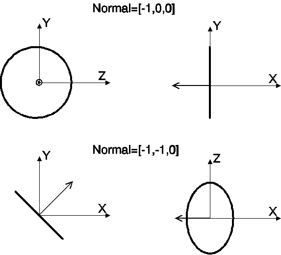
Figure 7 - Orientation Examples
For more general orientations, the region's normal can be specified to define the direction in which it faces. A normal of [0,-1,0] would put the region in the x-z plane (it's normal is parallel to the y-axis), and a normal of [-1,-1,0] would put the region parallel to the z-axis with its projection into the x-y plane a line with 45 degree angle.
Since the region is assumed to start in the y-z plane, care must be taken to specify the size correctly if another plane is desired. For example, for a rectangular region in the x-y plane with size in the x-direction of 10 cm and size in the y-direction of 5 cm, the orientation vector will be [0,0,1], but the size should be specified as 5,10 rather than 10,5, since the region will rotate around the y-axi s, moving the second number from z to x but leaving the first number as y.
A rectangle is specified by its center (or origin), its size in two dimensions, the sampling density on its surface (in each dimension), and its orientation in space. For the orientation given as an example above, the parameter file could be specified as either:
rectangle       ; Calculate within a rectangular section of space.
300,0,0         ; Origin (center) of rectangle
10,5            ; Size of rectangle (x_size=10, y_size=5)
0.5,0.25        ; Sampling density in x and y directions, respectively.
xy              ; Rectangle is in x-y plane.
or:
rectangle       ; Calculate within a rectangular section of space.
300,0,0         ; Origin (center) of rectangle
5,10            ; Size of rectangle (y_size=10, z_size=5)
0.5,0.25        ; Sampling density in y and z directions, respectively.
0,0,1           ; Rotate rectangle into x-y plane (normal is along z-axis.)
A curved rectangle is a rectangle which is curved in one dimension, that is, a section of a cylinder wall. The specified size of the rectangle in the curved dimension refers to the arc length, not the chord length. The radius of curvature of the rectangle may be non-zero in either the y or z direction, but not in both. A zero radius of curvature means a flat surface. If both radii of curvature are set to zero, then a curved rectangle is identical to a rectangle with the same parameters. An example parameter file section is:
curved          ; Calculate on a curved rectangular section of space.
300,0,0         ; Origin (center) of curved rectangle
10,5            ; Size of curved rectangle (y_size=10, z_size=5)
5,0             ; Curvature of rectangle (y_rad=5, z_rad=0 (flat))
0.5,0.25        ; Sampling density in y and z directions, respectively.
-1,0,0          ; Region's normal is in -x direction, so region lies in the yz plane.
The pressure field can also be calculated within a planar circle. In this case, the circle is specified identically to the rectangle, with the substitution of its radius for the rectangle's dimensions. An example:
circle          ; Calculate on a planar circle.
300,0,0         ; Origin (center) of circle
5               ; Radius of circle, in cm.
0.5,0.25        ; Sampling density in y and z directions, respectively.
0,1,0           ; Region's normal is in y direction, so region lies in the xz plane.
Focal Point Determination
The focal point of a lens system is defined as the point of maximum absolute pressure. The focal point can be found along a line or in a plane. The algorithm to find the focal point along a line is much faster than that for a plane, so should be used whenever possible. For searching along a line, the line is specified by its origin and angle in the y and z directions. The search range is given as distances from the origin along the line. If the line is parallel to an axis, then the appropriate angles can be set to zero, or a simplified form can be used. In the latter case, the axis which the line is parallel to is specified along with the fixed coordinates of the line in the other two dimensions. For searching in a plane, the corners of a rectangle within which to search, as well as the plane's identity, are given.
In all cases, a coarse search is done first over the search range in order to avoid local maxima, so the number of coarse search points must be specified. The maximum value of those found in the coarse search is chosen, then the maxima is refined until the accuracy condition is met. The accuracy is the distance, in cm, between the maxima and the nearest two search points. The algorithm used is a binary search, so the actual accuracy will be slightly higher than that given, depending on where the first subdivision which exceeds the specification lies.
Example parameter file for searching along a line:
line_max        ; Find maximum along a line.
300,0,0         ; Origin of line.
25.0,100.0      ; Search range along line (distances from origin).
30,0            ; Angle of line from x-axis (in y and z directions)
31,0.001        ; Number of coarse search points, maxima accuracy
Example parameter file for searching along a line which is parallel to an axis:
axial_max       ; Find maximum along a line parallel to an axis.
x               ; Axis which line is parallel to.
2.0,3.5         ; Fixed coordinates (in this case, y and z) of line.
25.0,100.0      ; Search range along line.
31,0.001        ; Number of coarse search points, maxima accuracy
Example parameter file for searching in a plane:
dual_axial_max  ; Find maximum in a plane.
xy              ; Use xy plane
5.5,0.0         ; Initial guess for y, fixed value of z.
320,400         ; Search range in x-direction.
2.5,8.5         ; Search range in y-direction.
31,0.001        ; Number of coarse search points, maxima accuracy
The planar algorithm finds the maximum parallel to the first axis at a fixed distance from the second axis (given by the initial guess.) Then it uses that point as the fixed distance from the first axis, and searches parallel to the second axis. This is repeated until the given accuracy is achieved. When searching along a ridge, however, this algorithm is very slow to converge. Therefore, when the maximum is known to lie along a certain line, it is much faster to use the line_max or axial_max routines.
The parameter file to describe any calculation ends with the element description. For a point element, this is simply the string "point". For more complicated elements, more description is required.
For a point element:
point ; Use a point element.For a rectangular element:
rect            ; Use a rectangular element.
1.0,0.5         ; Element is 1.0 cm high (y) and 0.5 cm wide (z)
For a line element:
rect            ; Use a rectangular element.
1.0,0.0         ; Element is 1.0 cm high but has zero width.
For a curved rectangular element:
curved          ; Use a curved rectangular element.
1.0,0.5         ; Element is 1.0 cm high (y) and 0.5 cm wide (z)
10.0,0.0        ; Radius of curvature of 10 cm in the y-direction.
For a circular element:
round           ; Use a round element.
1.5             ; Element's radius is 1.5 cm.
Element Pose and Sampling Density
For any element except a point element, the element's orientation and sampling density must also be specified. The element can be oriented in one of two ways: so that it is always facing a specified direction, or so that is always faces a specific point, regardless of the element's position. The number of samples taken on the element's face must also be listed.
Two examples:
point ; Element will always face the same point.5000,0,0 ; That point is (5000,0,0).
10 ; Number of points on element.
direction ; Element will always face in the same direction.
-1,0,0 ; That direction is the -x direction.
25 ; Sample 25 points on the element.
![]() Go back to the Example Lens System
Go back to the Example Lens System
![]() Go to the Utility Program Section
Go to the Utility Program Section
kevin@fink.com