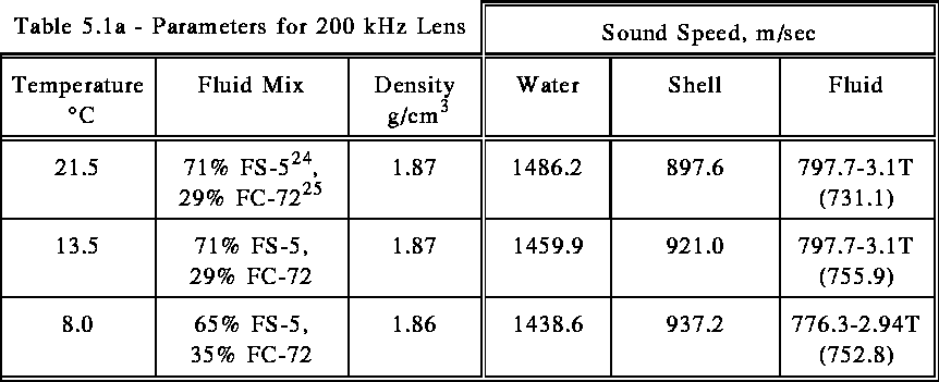
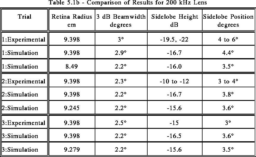
Figure 5.1 - 200 kHz Diver-Held Sonar Lens
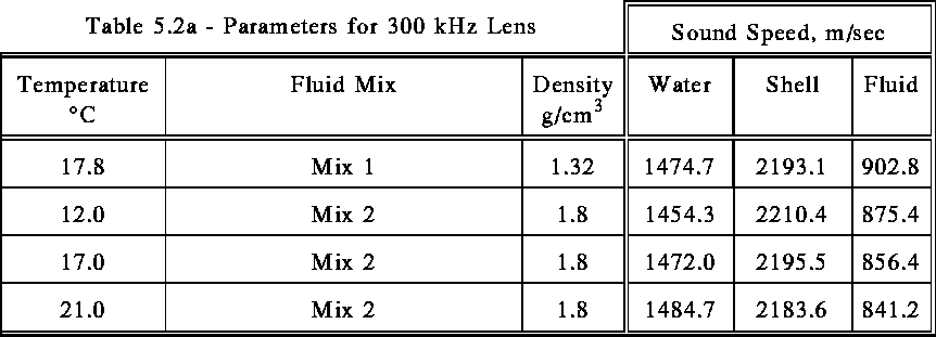
The first lens was designed for a diver-held sonar with 3 degrees beams operating at 200 kHz 6. It consists of a spherical rubber shell of inner radius 7.366 cm and outer radius 11.176 cm. The speed of sound in the shell is described by the equation 960.6-2.93T m/sec, where T is the ambient temperature in degrees Celsius. The retina radius was fixed at 9.398 cm; and the element was round with diameter 0.3175 cm. The shell could be filled with different mixes of liquids to provide appropriate focus for different temperatures. The parameters for the three trials that were run are tabulated in Table 5.1a.
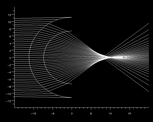
A comparison of the results from the simulation are compared to the experimental data in Table 5.1b. The focal points shown were found by the simulation; experimentally determined focal points were not available. Two beam patterns were calculated for each trial. The first used the same retina radius (9.398 cm) as the experimental configuration. The second used the focal point which the simulation determined for the retina radius.
The experimental data was taken from printed plots and could only be read to about 0.5 degrees accuracy for the beam widths, 1 dB accuracy for the sidelobe heights, and 1 degrees accuracy for the sidelobe positions. For all three trials, the simulated beam widths were within 0.3 degrees of those experimentally determined and the sidelobe positions were within 1 degrees of those experimentally determined. The sidelobe heights for the first and third trials were within 3 dB of the experimental data, but the second trail was off by between 5 and 7 dB.
The experimental data suggests that the second trial wasn't well focused (resulting in the large sidelobe level) due to using the summer fluid mix at a too-cool temperature of 13.5 degrees C. The simulation doesn't predict this problem, however.
The simulation predicts nearly identical results for all three trials if the retina radius is set to the focal point instead of being fixed at 9.398 cm. Thus changing the fluid mix and the retina radius can adapt the lens system to a wide temperature range with little or no degradation of performance. It would be interesting to see if this prediction held up in an experimental trial.
Figure 5.2 - 300 kHz Autonomous Underwater Vehicle Lens
Due to the thinness of the shell in this case, the ray tracing procedure may not accurately model the sound propagation. Looking at the ray trace plots, the geometrical acoustics predicts that a large proportion of the lens aperture completely blocks (or reflects) the incident sound. This is almost certainly not the case physically, but the appropriate model is not known at this time.
In order to match the empirical results more closely, trials were run approximating the shell as an infinitely thin interface with radius 11.176 cm (the inner radius of the actual physical shell) and 11.887 cm (the outer radius of the physical shell). It has also been found in previous experiments that using an effective aperture of 80% of the actual lens radius results in closer agreement with experimental results, so that was tried as well. Ray theory predicts that no rays will pass through an interface if they impact it at more than some critical angle. This critical angle prediction is not true in reality, and thus the simulation results in incorrect predictions. The 80% effective aperture represents a compromise between the true thick shell, which can not be modelled by geometric acoustics and a single interface with the same aperture as the thick shell.
In all cases the element was modelled as a square with 0.3175 cm sides, sampled 25 times, with uniform response over the face.
The results from all trials are tabulated below (Tables 5.2b through 5.2e). Note that the focal points for the experimental results are not measured values. They were calculated using the empirically derived thin shell formula 9
where
 is the speed of sound in water,
 is the speed of sound in the lens fluid,
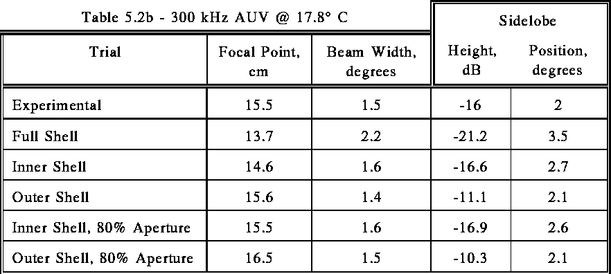
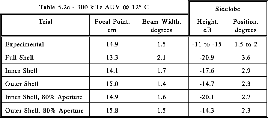
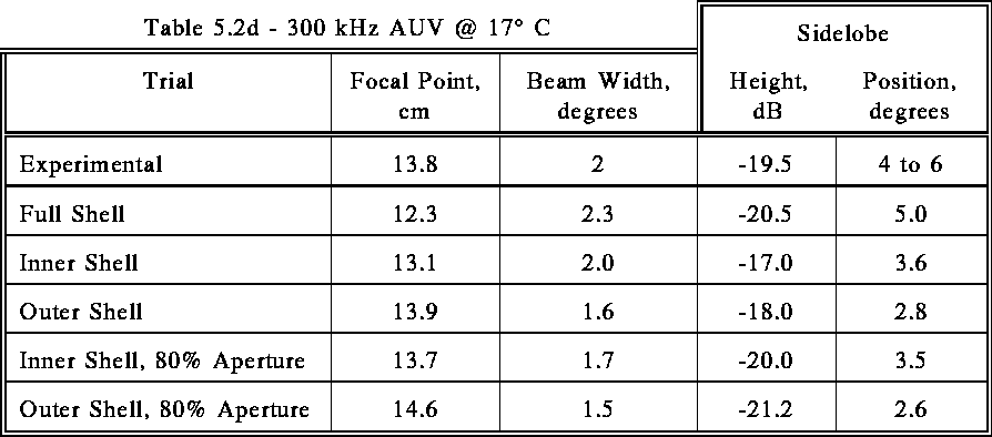
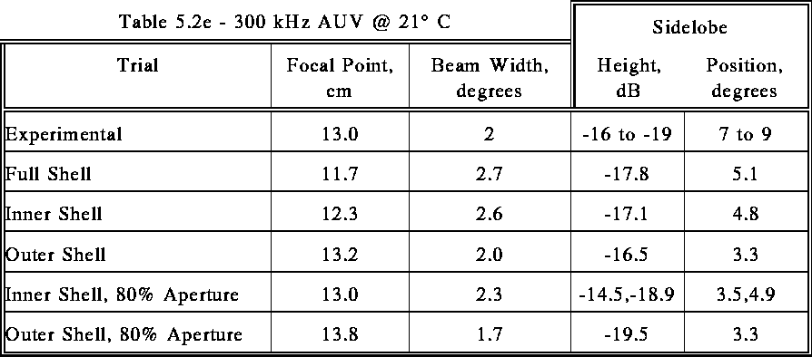
The simulations using the shell material showed larger beam widths, lower sidelobes, and closer focal distances than the experimental data. The zero-thickness shell simulations' predictions were closer to matching. The simulations using the outer shell and the inner shell with 80% aperture were the closest in all cases to the experimental data. The inner shell 80% aperture focal distances were identical to those predicted by the thin shell formula, and the beam widths were all within 0.5 degrees , which is as accurately as the experimental data can be read. The simulated sidelobes tended to be lower and positioned farther away from the main lobe than they were in the experimental data, but were not dramatically different in any case.
Figure 5.3a - 100 kHz Surveillance Sonar Lens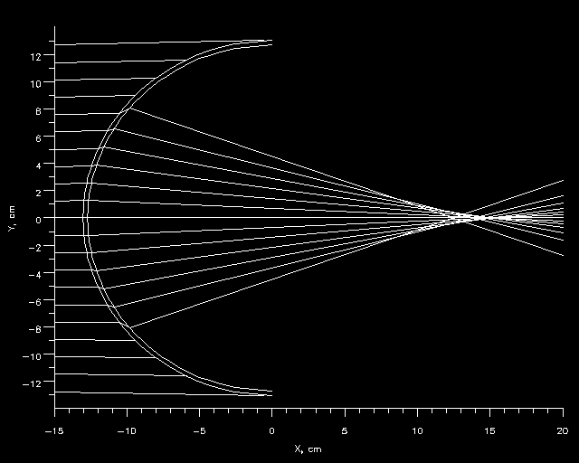
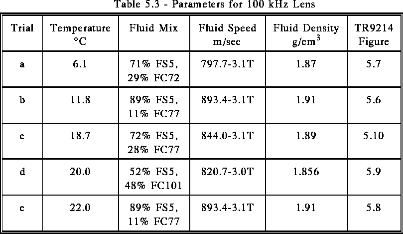
The simulations using the full shell did not agree well with the experimental data (Figures 5.3b and 5.3c, for example). The ray trace plot (Figure 5.3a) shows that the lens shell causes many of the rays to be discarded due to exceeding the critical angle condition. The critical angle condition is a prediction of geometric acoustics but not wave acoustics and thus is not accurate in all cases.
In order to better match the experimental results, the lens shell was modelled as an infinitely thin interface with radius equal to the inner radius of the physical shell. Simulations were run with lens apertures of 100%, 90%, and 80% of the physical aperture to approximate the shading of the true shell. These simulations matched the experimental results much better. In general, the 100% aperture simulations predicted a focal point just inside of the experimentally determined focal point and a smaller focal depth than the experimental data suggested. The simulated focal point moved out and the focal depth increased with decreasing aperture size. The 90% aperture trials seemed to match the experimental data most closely (Figures 5.3b and 5.3c). For some trials, though, the focal point was shifted by up to 1 cm (Figure 5.3c). The reasons for this have not yet been determined.
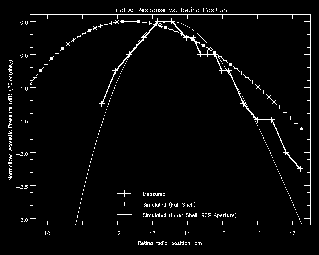
Figure 5.3b - Trial A: Focal Depth Results
Figure 5.3c - Trial D: Focal Depth Results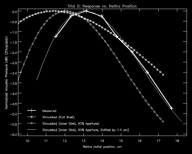
Many of the system parameters cause definite, repeatable changes in the pressure fields and beam patterns of lens systems. For example, if a lens system is to be used at several temperatures, it is useful to know how its performance will be affected by varying temperature. ALSSP is useful in investigating these effects.
Increasing the ambient water temperature moves the focal point of a lens system in and decreases the depth of focus. Figure 5.4.1a is a contour plot of the pressure field behind the lens described in section 5.3. The lens was simulated using the full shell, the operating frequency was set to 100 kHz, and the ambient water temperature was 6.1 degrees C.
After changing the ambient water temperature to 20 degrees C (Figure 5.4.1b), the focal point shifted from 12.2 cm to 10.8 cm (a -12% change), and the depth of focus (distance between the 3 dB points in the radial direction) decreased from 11.4 cm to 8.4 cm (a -26% change). The change in the focal point is much less than the focal depth at either temperature, so a retina position could easily be chosen that would provide good results at either temperature. In fact, the compromise retina position of 11.4 cm is only 0.1 dB down from the peaks of the two focal points.
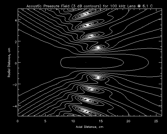
Figure 5.4.1a - 3 dB Contour Plot of Trial A: 100 kHz, 6.1 degrees C
Figure 5.4.1b - 3 dB Contour Plot of Trial A: 100 kHz, 20 degrees C
Increasing the operating frequency of a lens system changes the pressure field drastically. The entire field appears to be compressed and shifted out at higher frequencies. This moves the focal point out and decreases the focal depth. In terms of beam patterns, the beam width decreases with increasing operating frequency and the sidelobes move in. Sidelobe heights aren't greatly affected, but do tend to decrease slightly. To a first approximation, the pressure field is scaled by the frequency, so changing from 100 kHz to 300 kHz will compress the pressure field by a factor of 3.
Figure 5.4.2a shows the pressure field of the same lens as Figure 5.4.1a, but operating at 300 kHz instead of 100 kHz. The focal point moved from 12.2 cm to 13.9 cm (a 14% change), and the depth of focus decreased from 11.4 cm to 4.5 cm (a -61% change).
Figure 5.4.2a - 3 dB Contour Plot of Trial A: 300 kHz, 6.1 degrees C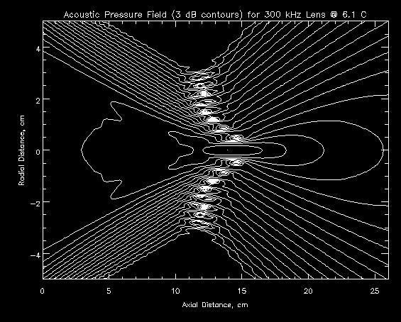
Figure 5.4.2b shows beam patterns for the system operating at 6.1 degrees C for the two operating frequencies. The retina radius was set to the focal point of system in each case. The beam width decreased from 5.1 degrees to 1.6 degrees (a - 69% change) and the sidelobe heights decreased slightly, from -13.5 dB to -14.1 dB (a -4% change).
Figure 5.4.2b - Effect of Frequency on Beam Patterns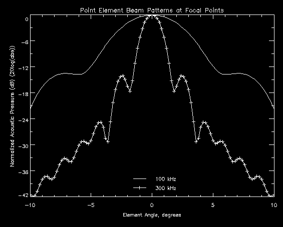
The effects of changing temperature are more drastic at higher frequencies because the pressure field is compressed. Figure 5.4.2c shows the pressure field for the lens operating at 300 kHz and 20 degrees C. The focal point moved in from 13.9 cm to 11.6 cm (-17%) and the focal depth decreased from 4.5 cm to 3.2 cm (-29%). The compromise retina position of 12.7 cm is 1.2 dB down from the peaks rather than the 0.1 dB of the 100 kHz system. The 300 kHz lens system will thus be much more sensitive to water temperature than the 100 kHz system.
Figure 5.4.2c - 3 dB Contour Plot of Trial A: 300 kHz, 20 degrees C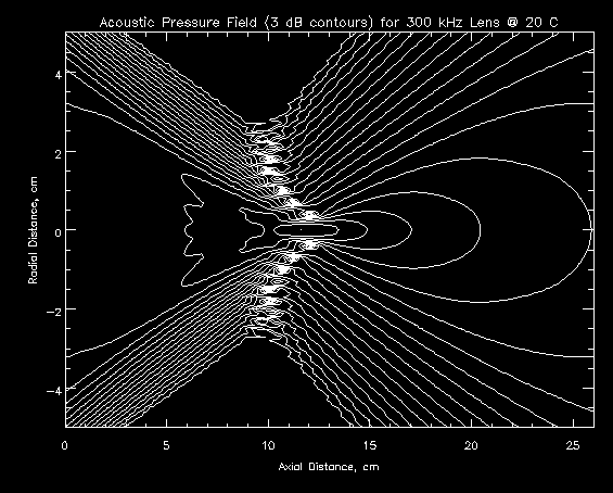
Introducing an element into a pressure field is equivalent to performing a convolution of the pressure field with an element function. For a point element, the pressure field is convolved with an impulse function, and thus is not changed. Therefore, the position of maximum response of a point element is the focal point of the lens system. For a larger element, however, the element function has larger support and the pressure field is "smoothed". Because of this, the position at which the element responds most strongly to the pressure field (the apparent focal point) will not be at the system's focal point. Increasing the element size moves the apparent focal point out and increases the apparent depth of focus. Figure 5.4.3a compares the response of a point element, a 1.0 cm diameter element, and a 2.0 cm diameter element moving along the x-axis of a lens system.
Increasing the element size also increases the beam width and decreases the sidelobe heights of beam patterns. Figure 5.4.3b compares the beam patterns of lens system using a point element, a 1.0 cm diameter element, and a 2.0 cm diameter element. The beam width increases from 3.1 degrees to 3.4 degrees to 5.0 degrees and the sidelobes drop from -10.8 dB to -11.7 dB to about -17 dB.
Figure 5.4.3a - Effect of Element Size on Axial Response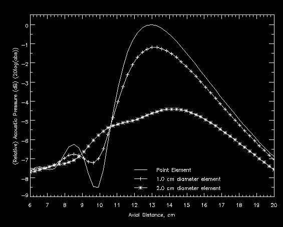
Figure 5.4.3b - Effect of Element Size on Beam Patterns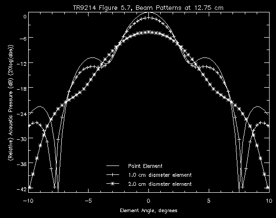
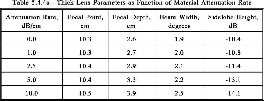
Sound attenuation in the lens material has the effect of "shading" the aperture. Lens materials often have much higher sound attenuation rates than the surrounding water or the lens fluid. In addition, rays farther from the lens center travel a longer distance through the lens material than those close to the center, and thus are attenuated even more. The magnitude of sound coming from the edges of the lens, then, is less than that from the center. This has the effect of moving the focal point out from the lens system and increasing the depth of focus. It also widens beam patterns, increasing the beam width and moving the sidelobes out. The height of the sidelobes is also reduced. Table 5.4.4a shows parameters for the 200 kHz lens described in section 5.1 with no attenuation in the shell material, 1.0 dB/cm attenuation, 2.5 dB/cm attenuation, 5.0 dB/cm attenuation, and 10.0 dB/cm attenuation. The focal point isn't greatly affected, but the depth of focus and beamwidths are strong functions of the attenuation rate.
The actual attenuation rate in the shell material for the 200 kHz lens is not known. However, similar materials have attenuation rates in the vicinity of 2 to 6 dB/cm. The response of the lens with 10 dB/cm attenuation is 40 dB lower than that with no attenuation, which would result in undetectable signal levels. Since the lens did in fact focus sound into detectable levels, the attenuation rate must have been much smaller than 10 dB/cm.
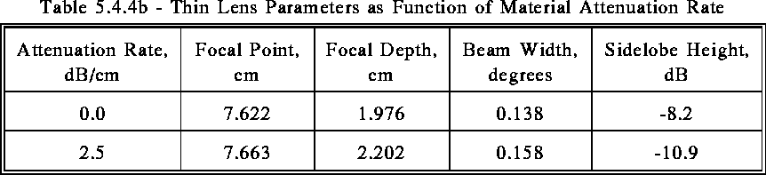
The effect of attenuation in the lens material is much more pronounced in the case of thin lenses, since they are generally thicker near the edges than near the center. Table 5.4.4b shows that changing the attenuation rate from 0.0 to 2.5 dB/cm for a thin lens changes the beam width by 14% and the sidelobe height by 33%, whereas the respective changes were only 11% and 10% for the same attenuation rates in the thick lens. The focal depth changed by about the same percentage (10%) in both the thick and thin lens cases.
Incorporating sound attenuation is theoretically sound, but requires knowledge of the sound attenuation rate in each material. This is generally a function of frequency and temperature, and may not be readily available. In addition, for thick lenses, incorporating sound attenuation requires the use of a shell. In some cases that may cause problems (see section 5.3), so an alternate method is used.
Decreasing the aperture size of a lens system is one way to approximate the attenuation of the lens material without requiring a shell and knowledge of the sound attenuation rate in the shell. It is equivalent to making the attenuation rate infinite beyond a certain radius of the lens, while not changing it within that radius. Reducing the aperture of a lens system often helps make a simulation agree with experimental results, but doesn't have as strong a justification as incorporating the attenuation rate of the lens material.
Decreasing the aperture moves the focal point out, increases the depth of focus, widens beam patterns and modifies sidelobe heights and positions. Since sidelobes are effects of interference between the virtual point sources on the final lens surface, the change in their heights doesn't follow a simple rule. Table 5.4.5a shows the parameters of the 200 kHz lens system described in section 5.1 at 100%, 90%, and 80% of full aperture. Figure 5.4.5 shows beam patterns for the same system.
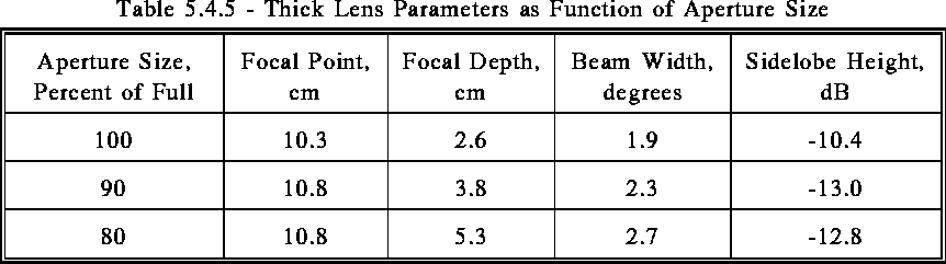
Figure 5.4.5 - Effect of Aperture Size on Beam Patterns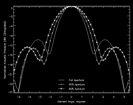
To illustrate the use of ALSSP in an iterative design project, a thin lens system has been designed that is to operate at 900 kHz in 10 degrees C fresh water. The beams formed should be less than 0.25 degrees wide with sidelobes more than 40 dB down within a 10 degrees field of view, and less than 0.5 degrees wide with sidelobes more than 20 dB down within a 50 degrees field of view. The element size and positioning need to be determined in order to finish the system design. For a more complete explanation of the commands required to execute this example, see the ALSSP User's Guide
The first step in setting up a lens system is to build the system parameter file. This lens system was designed using BEAM THREE, so the OPTICS file, which contains the lens interface and material information, is available.
GENERATE_SYSTEM will convert the OPTICS file to a form that CALC_LENS can use. However, BEAM THREE only does ray tracing, so does not provide information about the system frequency or the ambient conditions. The frequency (900 kHz), water salinity (0 parts per thousand), water depth (1.0 meter), water density (1.0 g/cm3), rate of sound attenuation in water (0.0 dB/cm), and the number of rays to trace (301) will be stored in a system header file 'system_header'.
In order to decide where elements should be placed, the focal point of the system for various source angles must be found. GENERATE_SYSTEM will make parameter files to do this automatically if given the desired source angles. Source angles of 0 degrees , 1 degrees , 2.5 degrees , 5 degrees , 10 degrees , and 25 degrees will provide a good picture of the retina shape. In addition, the point source distance must be defined. For this lens system, the targets will be approximately 25 meters from the lens, so the point source will be positioned 25 meters from the first lens surface. The lens material used is syntactic foam, which has a sound attenuation rate of approximately 1.0 dB/cm at 900 kHz.
Figure 5.5a - Thin Lens System with Focal Trajectory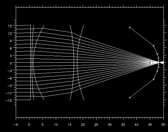
In Figure 5.5a, the lens system is the five curved surfaces on the left and the retina is the plus symbols connected by line segments. The left-most lens element is an iris, implemented as a planar surface that doesn't affect the rays except to define the aperture of the system. The iris could be eliminated by setting the first lens interface's aperture to the diameter of the iris, but GENERATE_SYSTEM takes the interfaces directly from the OPTICS file, so it is included as a separate element.
The next two surfaces represent the first syntactic foam lens. The first is an oblate ellipsoid, the second a hyperboloid. The final two surfaces are a second syntactic foam lens. The front surface is another hyperboloid and the back surface is a prolate ellipsoid.
The focal points found for each source angle are shown as plus symbols ('+') in the figure, and are joined by line segments to approximate the ideal retina shape for the lens system. Note that this system is symmetric about the x-axis, so the focal points found for positive source angles can be mirrored for the corresponding negative source angles.
The next step in analyzing the system is to compute beam patterns. The program MAKE_BEAMS2 will be used to generate the parameter files to do this. Since the retina is not an arc, the element must be moved along a trajectory approximating the retina shape. However, the retina can be approximated as a collection of arcs for small changes in the source angle. The center of each arc is referred to as the secondary principal point in optical lens design. The program FOCI_CIRC1 finds the parameters of these arcs.
Representative two way beam patterns (the complex pressure is squared in order to simulate a lens system used for both transmitting and receiving) are shown in Figures 5.5b and 5.5c. The numerical results are tabulated in Table 5.5a.
Figure 5.5b - Beam Pattern for On-Axis Point Source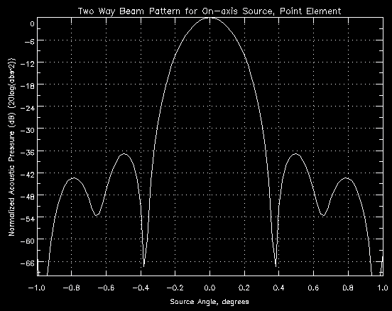
Figure 5.5c - Beam Pattern for 25 degree Off-Axis Point Source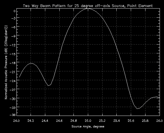
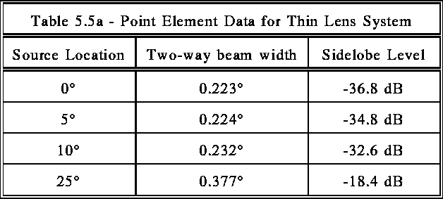
Table 5.5a shows the beam widths are all within the specifications, but the sidelobe levels are all too high. However, these calculations were made for a point element. Any real element will have a physical size and shape that will affect the beam widths and sidelobe levels. By adding the effect of element size and shape into the calculations, the sidelobe levels can be decreased for a small penalty in beam width. For example, adding a 0.268 cm element results in similar beam patterns, but ones that exhibit slightly larger beam widths and lower sidelobe levels, as expected. The results are tabulated in Table 5.5b:
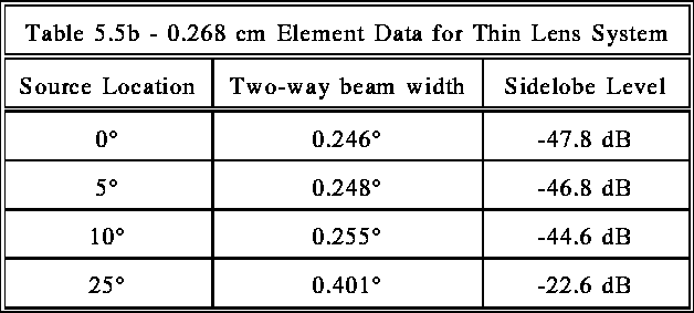
Now the specifications have been met. For the 10 degrees field of view, the beam widths are under 0.25 degrees and the sidelobe levels are below -40 dB. For the 50 degrees field of view, the beam widths are under 0.5 degrees and the sidelobe levels are below -20 dB.
kevin@fink.com